|
Oscilloscope |
  
|
|
Oscilloscope |
|
Overview:
The oscilloscope is used to visualize a device's signals and allows monitoring two devices simultaneously, with up to 4 channels each. The maximum sampling rate is 2000 measurements per second (500 μs) per channel. An Ethernet cable connection must be used with the device (e.g., CFW900), and it is not necessary to "Connect the Device" in the top menu of the WPS. To monitor two devices simultaneously, a daisy-chain connection is required (Computer -> Device Name -> Device Name), utilizing both Ethernet ports of the device.
The oscilloscope can be found in Window > Oscilloscope.
1) Top bar:

| • | 1: Starts monitoring. |
| • | 2: Stops monitoring. |
| • | 3: Resumes monitoring. |
| • | 4: Pauses monitoring. |
| • | 5: Clears measurements from the graph. |
| • | 6: Increases zoom while maintaining horizontal position. |
| • | 7: Decreases zoom while maintaining horizontal position. |
| • | 8: Adjusts vertical zoom based on measurements. |
| • | 9: Adjusts zoom based on data, horizontal and vertical. |
| • | 10: Enables a cursor to measure values from the graph. |
| • | 11: Enables two cursors to measure values from the graph, including time difference. |
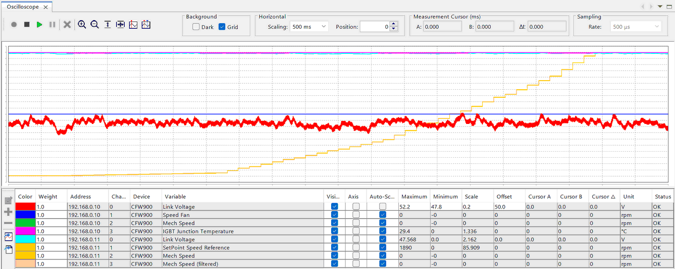
| • | 12: Visual configuration of the table. The left selector activates the dark mode for the chart, and the right one enables the grid lines. |
| • | 13: Scale of the graph divisions; in this case, each vertical grid division will be 500 milliseconds. |
| • | 14: Position of the horizontal axis. |
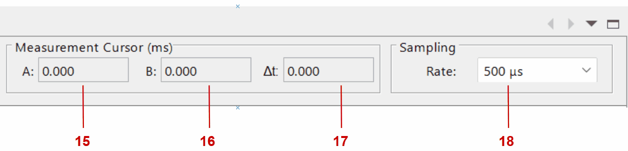
| • | 15: Value of the first cursor (red) on the X-axis in milliseconds. |
| • | 16: Value of the second cursor (blue) on the X-axis in milliseconds. |
| • | 17: Delta (difference) between the values of the first and second cursor. |
| • | 18: Sampling rate; it defines the interval between measurements sent by the device; in this example, 2000 measurements will be sent per second. |
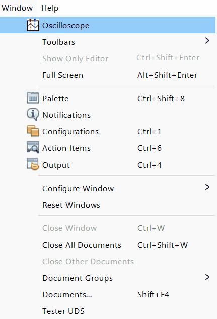
2) Bottom table:
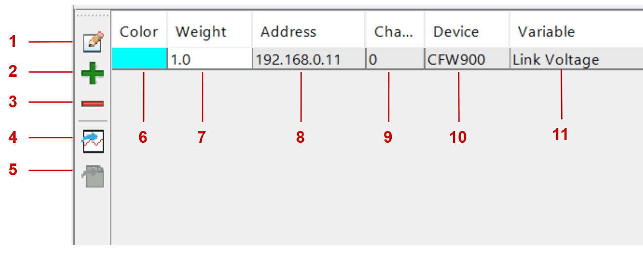
| • | 1: Device editor. |
| • | 2: Add devices. |
| • | 3: Remove devices. |
| • | 4: Import data. |
| • | 5: Export data. |
| • | 6: Channel color indicator/selector. |
| • | 7: Channel thickness indicator/selector in the graph. |
| • | 8: Device IP on the Ethernet network. |
| • | 9: Channel ID. |
| • | 10: Device model. |
| • | 11: Variable name. |
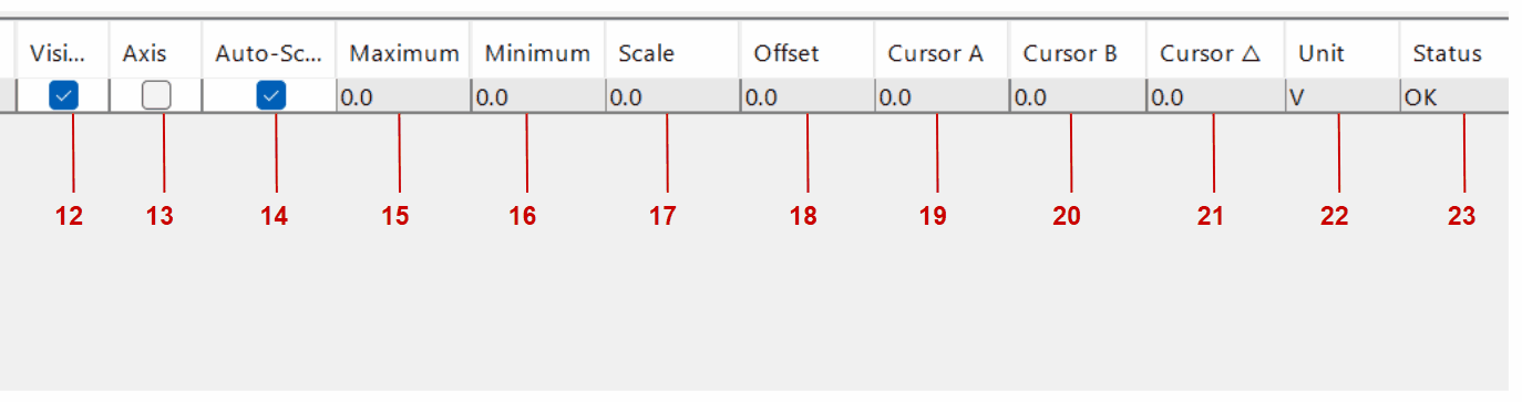
| • | 12: Makes the channel visible or not visible. |
| • | 13: Enables the Y-axis related to the channel for easier visualization. |
| • | 14: Enables Auto-fit (Auto-scaling); this uses the received maximum and minimum values to define the Y-axis limits of the channel. |
| • | 15: When auto-scaling is disabled, it allows setting the maximum value of the Y-axis of the channel. |
| • | 16: When auto-scaling is disabled, it allows setting the minimum value of the Y-axis of the channel. |
| • | 17: Multiplies the maximum and minimum values, defining the size of the vertical divisions. |
| • | 18: Determines the vertical position of the channel; it is not relative to the signal. For example, a sine wave varies from 0 to 100; an offset of 50 places the signal exactly in the center of the graph. |
| • | 19: Channel value at the position of the first cursor (red). |
| • | 20: Channel value at the position of the second cursor (blue). |
| • | 21: Difference between the measurements of the cursors. |
| • | 22: Unit of the variable chosen for the channel. |
| • | 23: Connection status with the channel. |
3) Device configuration page:
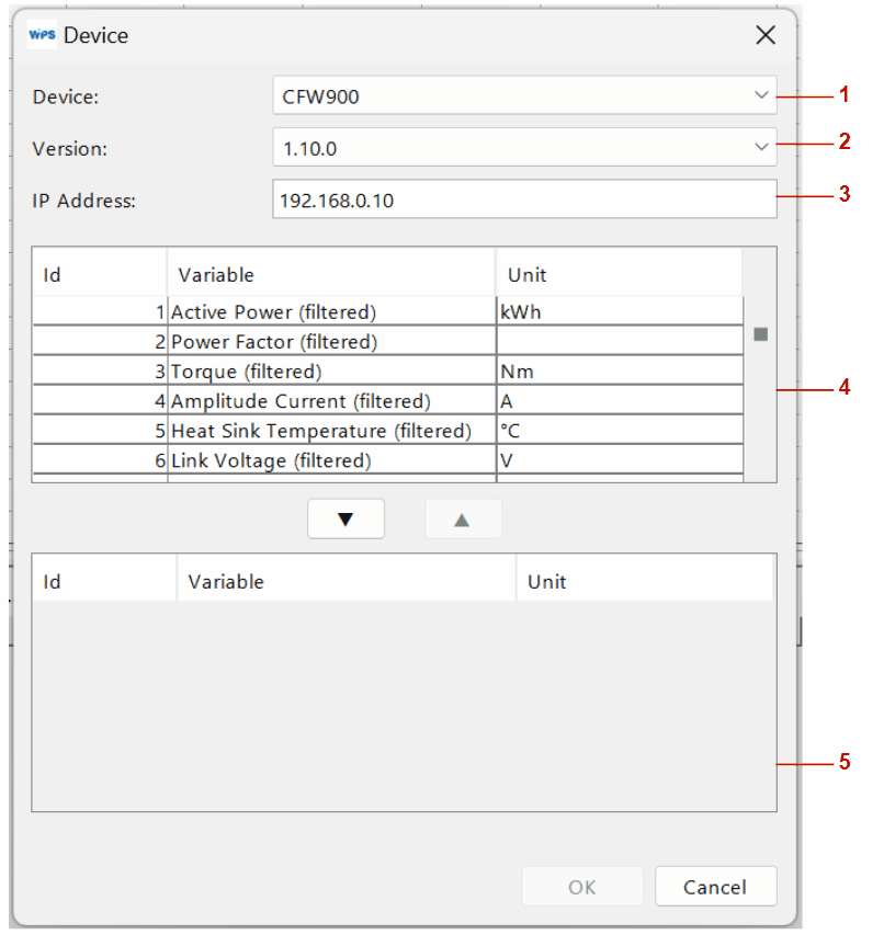
| • | 1: Device model (if supported). |
| • | 2: Controller firmware version. |
| • | 3: Controller IP address. |
| • | 4: List of parameters available for monitoring. |
| • | 5: List of selected parameters; to insert or remove items from this list, simply select from the upper list and use the arrows to move between lists. This list defines the channels of the oscilloscope. |
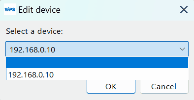
4) Modify a device:
The device modification screen is the same as the device addition screen. By clicking the button (item 2.1 of this document), you can select a device and modify it.
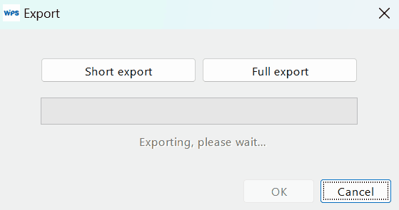
5) Export Data:
The data export screen offers two options:
Partial Export: exports the last 20,000 data points, faster.
Full Export: exports all data since the start of recording; may take a long time due to the volume of data.
Functionalities:
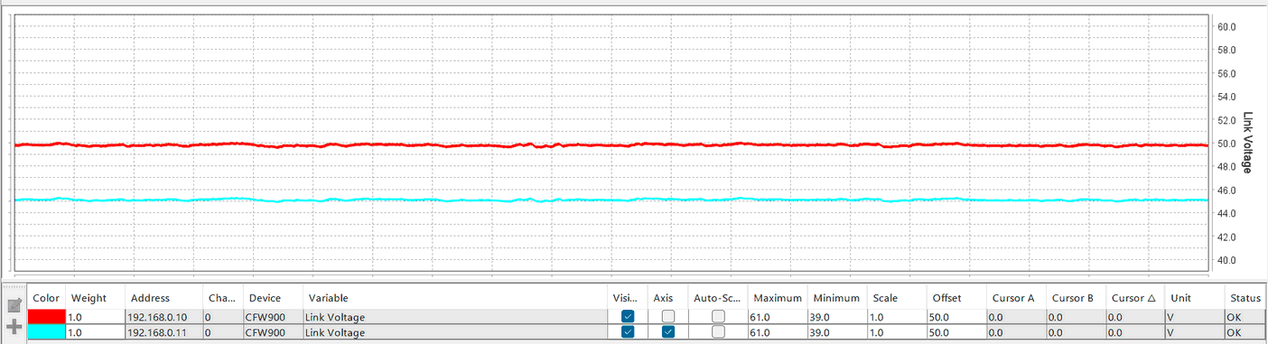
Offset:
The offset configuration is useful when we want to move a channel vertically, such as comparing a variable from two different devices. We can observe that both channels have the same maximum, minimum, scale, and offset values, but still do not overlap.
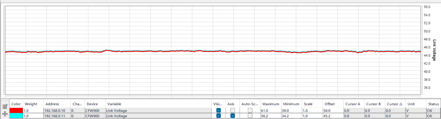
We can correct this by adjusting the offset, in this case from 50 to 45.2. To identify the ideal offset value, it is recommended to use the channel scale as a reference for values. It is worth noting that the offset also changes the vertical limits of the graph.
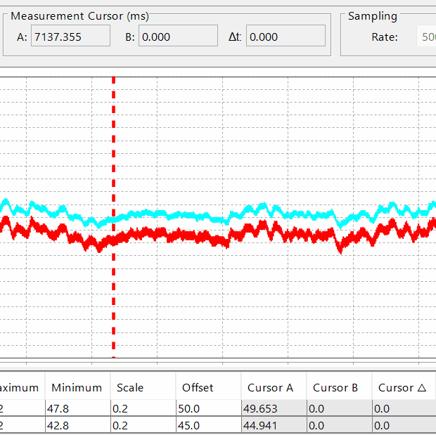
Cursors:
To measure values more precisely than the channel scale, it is possible to use the cursors (with the graph paused or stopped). We have two options:
| • | Single cursor: only one cursor is used, useful in cases where it is only necessary to know the value at a certain point. At the top, in "Measurement cursor (ms)," we can see that cursor A is at position 7137.355, which means this point is 7469.864 milliseconds after the start of recording. At the bottom, in the "Cursor A" column, we can see the values of each channel at this point. |
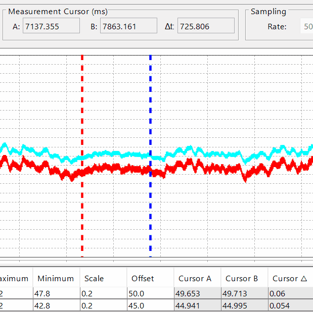
| • | Double cursor: Two cursors are used. Useful for checking the difference between two points, both in time and value. We can see that both at the top and bottom, we now have values in the field B (second cursor, in blue) and in the delta field, with field B showing the values at cursor B and delta showing the difference between them. |
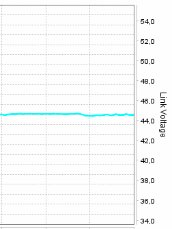
Channel vertical scale:
The scale determines the size of the vertical divisions, changing the maximum and minimum values of a channel. In cases where a channel has little variation in values, it can be used to improve visualization by adjusting the maximum and minimum values of the channel, effectively "stretching" the signal. In the following image, the channel is set with a scale of 1, so the distance between each horizontal line is one unit; however, with a signal that has little variation, it makes data visualization more difficult.
By changing the scale to 0.05, we achieve a zoom effect on the data, making visualization easier:
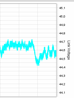
It is recommended to first correct the offset and then adjust the scale, or the signal may go out of the visualization range.
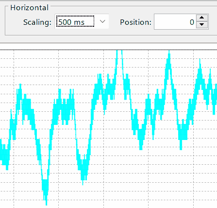
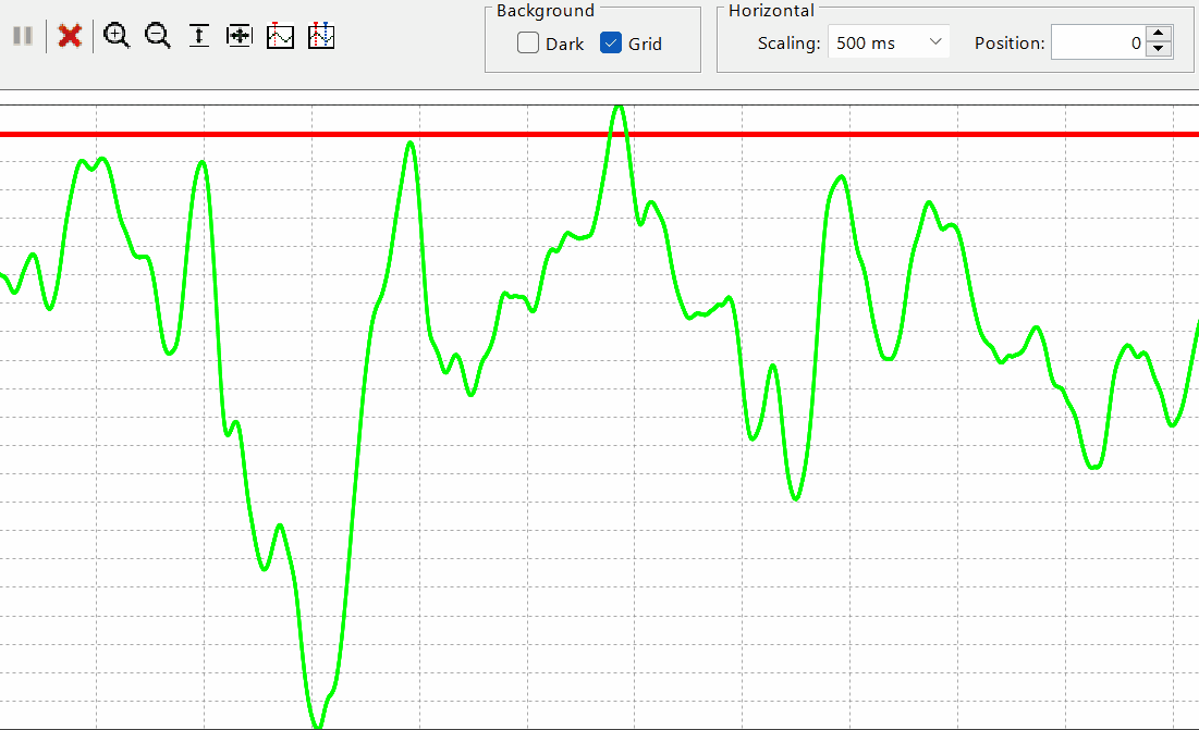
Horizontal scale of the graph:
The horizontal scale (item 1.13 of this document) is used to define the period between horizontal divisions. The larger the scale, the greater the period between divisions. In the following example, we have the scale set to 500 milliseconds with a sampling of 500 microseconds, resulting in one thousand samples per division:
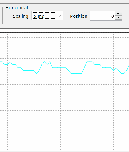
By changing the scale to 5 milliseconds, we have 10 samples per division, functioning as a horizontal zoom:
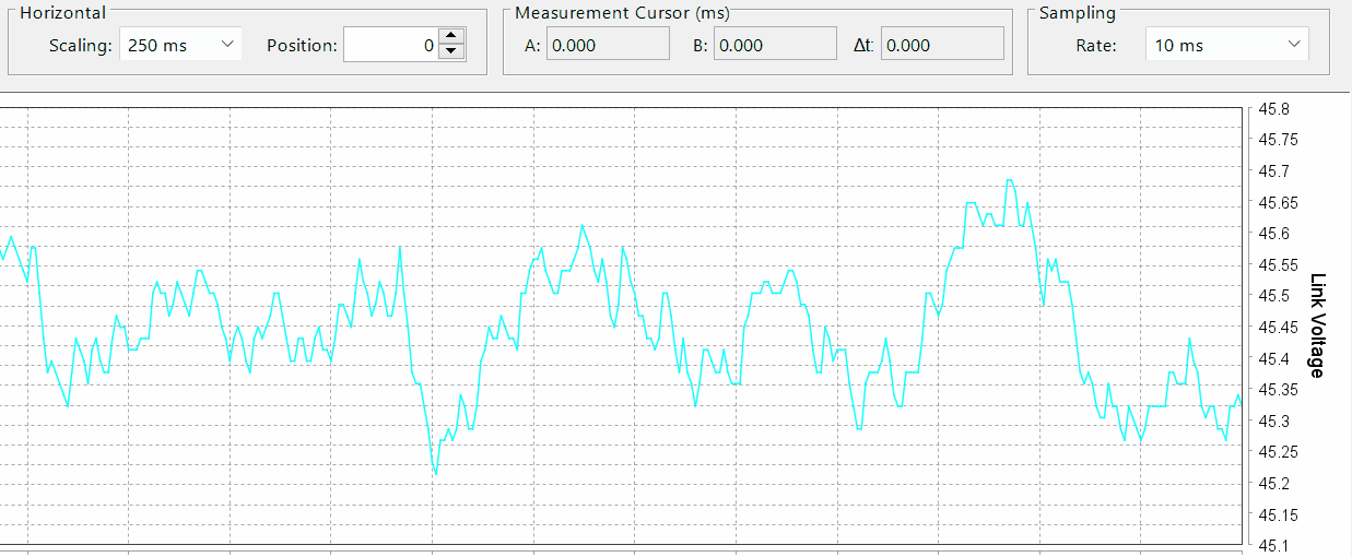
Sampling:
The sampling (item 1.18 of this document) defines the interval between the transmission of measurements from the device to the oscilloscope. A sampling of 500 microseconds results in 2000 data points per second, while a sampling of 10 milliseconds means 100 data points per second. The shorter the interval between samples, the more detailed the channel graph will be.
10 milliseconds Sampling:
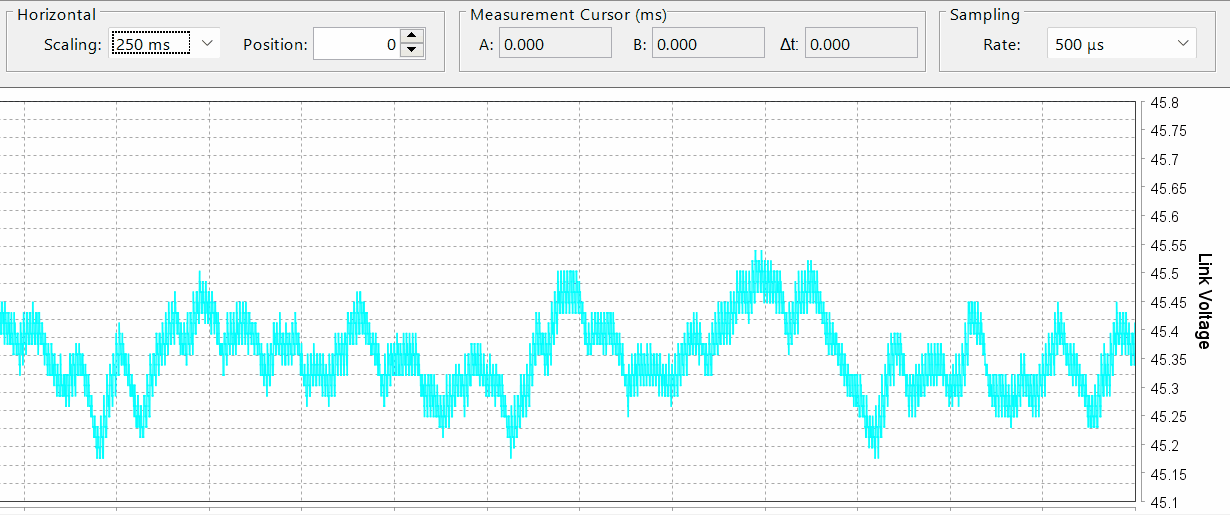
500 microseconds sampling:
Horizontal position:
The horizontal position controller (item 1.14 of this document) is used to move the time axis of the graph, enabling better visualization or comparisons. Its scale is based on the divisions of the graph; a shift of "1" will move the graph by one vertical division. Therefore, if the horizontal scale is set to 250 milliseconds, a shift of "1" will move the graph by 250 milliseconds.
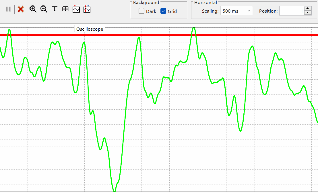
Position at 0:
Position at 1: